The most exciting developments of AI in 2018 is AutoML. It automates machine learning process. In January this year, Google released AutoML Vision. Then in July Google launched AutoML for machine translation and natural language processing. Both packages have been used by companies such as Disney in practical applications.
Google’s AutoML is based on Neural Architecture Search (NAS), invented in the end of 2016 (and presented in ICLR 2017) by Quoc Le and his colleague at Google Brain. In this article I will review the historical context of AutoML and the essential ideas of NAS.
Historical context
In the last 6 years (since 2012), AI has taken the world by storm. The term machine learning has become an almost magic phrase, implying some process that can automatically solves problems that human cannot. Be it showing ads, making recommendation, or predicting a frauded transaction, machine learning has become the synonym to automation.
But in reality, machine learning process is still quite manual.
The manual process in machine Learning: Feature Selection
In statistical (“classical”) machine learning (such as Decision tree, SVM, and Logistic Regression), we select inputs for making prediction. For example, in order to predict how like a person buys a bottle of coke, we use inputs such as a person’s age, gender, income, and so on. In this process, we have to decide on relevant “features” to use. We may miss some important features, for example, location of this person. Ideally we can add many features into the model. But they can degrade the performance of the machine learning model. Not all features are relevant. Even if a learning method can accommodate a large number of input features, it is still a manual process to create input “features”.
The job of a data scientist is coming up with good features by looking into data, doing experiments, or interviewing experts.
For many decades in the field of computer vision, researchers tried to come up with good features to summarize a picture: contrast, brightness, color histogram, etc. Yet, searching for good features are illusive. With human-crafted features (inputs), the accuracy of image recognition hovers around 70%, and speech recognition barely crosses 80% accuracy in normal cases. The same goes with many other tasks.
Deep Learning: Automating Input Selection
The revolution of deep learning is removing one manual process: Feature selection. In image recognition, we feed the picture at the pixel level to the model, without worrying about what features are important. The “features” are captured in the hidden layers and in the connection strength. In machine translation, we feed the input sentence at word or even character level to the learning model, and it learns to spin out the right sequence of words in a different language.
Deep learning — the learning of deep neural networks — completely removes the need to construct “features” at the input level. For this reason, deep learning is universal and speeds up the model building process. After removing human in the loop, the accuracy of image recognition jumped from 72% to 83% in 2012 in the ImageNet competition, more than 10% absolute improvement in accuracy.
The manual process in deep learning: Deciding on the architecture of a neural network
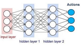
Despite its power and versatility, deep learning still has its manual process. Let’s take a look where the manual process comes from. Here is the stylized picture of a neural network.
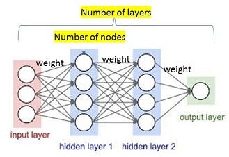
A neural network consists of neurons, layers, and activation functions. The connection strength among neurons are called weights, which are learned over time.
Architecture of a Convolutional Neural Network
A convolutional neural network consists of filters (for convolution operation), which determines the number of neurons in the next layer, and layers, and activation function.
A filter is a small square, such as 5×5. When applying this filter to the original image, we map a region of size 5×5 to a single point in the new image. Below is the picture to illustrate this:
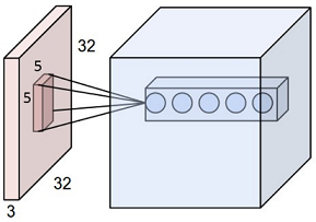
The original image has size 32×32, and our filter is 5×5. This maps a region of 5×5 in the first layer to a point in the next layer. There are total 5 filters (indicated by 5 dots in the second layer) :
Stride is the steps the filter moves on the image. When stride=1×1, the filter moves to the right by 1 pixel, and lower by 1 pixel. When stride=2×1, the filter moves to the right by 2 pixels, and lower by 1 pixel.
For a 6×6 image, we apply a filter 3×3 and use stride=1×1, we will get a 4×4 image.
Therefore deep learning still has human in the loop: Deciding on the number of layers, the filter size, stride size and the activation function.
The search for the best neural network architecture
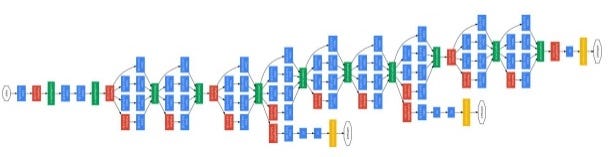
The evolution of deep learning field is corresponding to finding the best neural network architecture. In 2012, AlexNet has 8 layers, the winner of ImageNet competition in 2014 GoogleNet has 22 layers, and the winner in 2015 Resnet has 152 layers.
More layers and more parameters come with huge computational cost and slow down of training. Imagine a 100-layer neural network with 100 neurons at each layer, the number of connections between all neurons is 100²x100, or 1 million. In fact, Resnet has 1.7 million parameters. In other words, training a neural network is very expensive and slow. If you are doing experiments to find out how to build the best neural networks, you wait for several days or even weeks to get the result from 1 neural network. Then you add layers or number of neurons (in 1 layer), then you run the training again, waiting for a few more days.
On the other hand, we want to achieve high accuracy. Does that mean we have to increase the number of layers beyond Resnet? How many layers should we aim for? How many neurons (or filters) should we have in each layer?
Answering these question is equivalent to searching for the best architecture of a neural network: Deciding on the right number of layers and number of neurons. Since it is impossible to search exhaustively all parameters or configurations, due to the high cost of computing, we need a much more intelligent way to find the best architecture.
The Basic Ideas of Neural Architecture Search
Imagine we have an agent (controller) who tries to find out the best architecture (configuration) of a neural network. A neural network architecture can be described in a few parameters: The number of layers, the number of nodes etc. For a convolutional neural network (CNN), this is the number of filters and filter size. The controller can choose the size of these parameters.
1. Applying Reinforcement Learning to train the controller
In reinforce learning, an agent takes an action, observes reward. If an action leads to better reward, the agent will take that action more often, while exploring new actions. After trying many possible actions, the agent will settle down to 1 action that leads to the highest reward.
The controller now has a set of “actions”: Choosing the size of these parameters. Given the controller’s choice (actions), a neural network is created (but weight not yet assigned). This network will be then trained in the training data to get its weight updated.
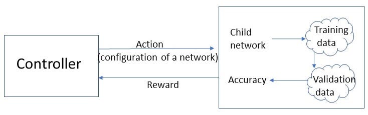
Once we make our choice, we have a specific network[1]. The performance of this network, measured in accuracy (on a test set or validation set), is our reward.
The goal is finding actions that lead to the maximal total reward when applying an action many times (or in different situations).
2. Using Policy Gradient Method: An Online Reinforcement Learning method
Traditional reinforcement leaning uses Q-value to track the performances of different actions. Q-value is the sum of expected reward when the agent takes the best actions. This requires trying a large number of actions and jumping through different reward outcomes. Thus the search is very slow. Instead, we can directly learn the impact of the action by observing the shift of current reward. This the idea behind policy gradient. The term “gradient” means moving along the steepest slope of the possible total reward.
When we use a neural network to learn the actions, we have what is called policy gradient network, or policy network. This is used by AlphaGo, thus receiving a lot of attention recently.
A policy network assigns probability of each action. The network updates its weights based on the gradient of the change of expected reward. For example, if you have 4 actins to take, each has 0.25 probability, the action output will be [0.25, 0.25, 0.25, 0.25], with T times of sampling based on this action distribution, you receive some rewards. Then get the sum of these rewards, and then update the weights of neural network (policy) based on the gradient of these rewards.
I will skip the elaborate mathematics on deriving this formula, but the essence is each weight is updated based on the derivative of Log function on the total reward.
The Controller is a policy network
The controller itself is a policy network, generating a child network based on probabilities on each action. After receiving the reward, it updates internal weight. In essence, the reward is higher for child network that has higher accuracy, thus increasing its probability in the policy network (to be chosen next time).

The neural network in the controller is a recurrent neural network, allowing flexible number of layers of the child network to be generated.
So far I have given a very high-level summary of the Neural Architecture Search and its historical context. For specific implementation, please refer to the original paper.
[1] This is called “child network” in the paper. The term “child” is actually very accurate. The controller (parent) create a blank network with certain number of nodes and layers, but all the weights are not yet trained. This network is then trained in the training data to update its weight, so that it performs well in the validation data.
References:
Barret Zoph and Quoc Le. “Neural architecture search with reinforcement learning.” arXiv preprint arXiv:1611.01578 (2016).
Quoc Le, Inventors of AutoML, is going to speak at AI Frontiers Conference on November 9 in San Jose, California.

AI Frontiers Conference brings together AI thought leaders to showcase cutting-edge research and products. This year, our speakers include: Ilya Sutskever (Founder of OpenAI), Jay Yagnik (VP of Google AI), Kai-Fu Lee(CEO of Sinovation), Mario Munich (SVP of iRobot), Quoc Le (Google Brain), Pieter Abbeel (Professor of UC Berkeley) and more.
Buy tickets at aifrontiers.com. For question and media inquiry, please contact: info@aifrontiers.com